Python Application for Oil and Gas Data Analysis
Transcript from Sumij Academy Presentation
Good morning and welcome to this first appointment.
Today we are talking about the Python application for oil and gas data to display and make analysis. My name is Matio. This appointment is in partnership with the Slumberj Academy.
We are focused on pressure and porosity monitoring in plastic reservoir and carbonate reservoir, estimate and plot clay volume, utility volume, plot volume of gas in different physical phase in plastic reservoir, analyze the composition in plastic reservoir in mixing zone, PVT calculation for gas plastic reservoir, create analytic tables for evaluating the incoming value for some companies.
For all kinds of these points, we will make example coding and analysis.
Pressure and Porosity Monitoring
Start with the first point: pressure and porosity monitoring in plastic and carbonate reservoir.
What do we mean when we are talking about pressure and porosity, especially in plastic reservoirs?
We have three different types of porosity and condition:
Interconnected porosity – pores with more than one throat connected to others. Hydrocarbon extraction occurs in this situation.
Suck or kinetic porosity – pores with one throat connected to others. Related to expansion in reservoir pressure.
Closed or isolated pore – closed pores, not connected to others. Not yielding hydrocarbons under normal processes.
Generally, we have a table summarizing the genetic condition involving the formation of gas in classic reservoirs. For example, in shallow zones with certain temperature ranges, we have grain coating and non-pervasive carbonate cementing, preserving initial porosity.
Other conditions that destroy porosity include clay infiltration, carbonate or silica cement, or autogenetic processes.
Porosity Evolution and Diagenesis
Intermediate temperature ranges lead to a medium state of dissolved carbonate. We might find feldspar, carbonate, quartz cement, and carbonate precipitation, which can destroy porosity. When temperature is too high, chemical precipitation is limited.
Compaction, cementation, and dissolution of certain minerals can affect porosity in sandstone reservoirs. This is the principal phenomenon in plastic reservoirs and influences porosity over the life of the reservoir.
Porosity origin and evolution depend on parameters like depth, original porosity, and natural or artificial processes such as fracturing. Natural porosity changes with processes like compaction, cementation, or clay matrix formation.
We distinguish between:
Primary porosity – original porosity from sedimentation
Secondary porosity – formed after compaction and diagenesis
Studying the history of plastic reservoirs is not only important to understand their formation but also to apply new techniques like machine learning to predict future evolution.
Using Machine Learning and Coding
Constant compaction causes porosity loss. In buried sandstone and shale, porosity changes over time. Understanding this helps justify the use of coding and machine learning to predict porosity and pressure evolution and to plan reservoir maintenance and safety operations.
Diagenetic stages (eogenetic, mesogenetic, etc.) can be analyzed by temperature phases and depth. For example, at depths beyond 2,000 m, we can see temperature changes of 16–17°C over reservoir life.
Reservoir Quality and Depositional Phases
Experience and Slumberj’s contribution help us classify different depositional phases and diagenetic alterations. For example:
In deltaic environments, grain coatings reduce permeability.
In shallow marine zones, strong vertical heterogeneity and better reservoir quality are observed.
These aspects connect geology and coding. Understanding geologic deposition helps us code better reservoir models.
Simulated Case and Porosity Forecasting
We simulate a delta environment and analyze:
Primary porosity – original
Secondary porosity – modified by compaction and diagenesis
We use Streamlit to simulate pressure and porosity over 5 years using initial porosity, pressure, compaction rate, and pressure decline.
In this delta case, porosity remains essentially constant while pressure declines—providing a good example of monitoring with code.
Pressure Monitoring in Carbonate Reservoirs
Pressure monitoring is critical for reservoir management and enhanced oil recovery. It helps plan operations and prevent damage from excessive compaction and subsidence.
We use logs like:
Density log – repeated multiple times during reservoir life
Neutron log – sensitive to hydrogen content
Sonic log – for porosity via travel time
We can also use MDT/FTT testing, production data, interference pulse tests, and pressure drop analysis.
If manipulating pressure artificially (e.g. fracking), careful planning is required, including environmental and seismic considerations.
Simulated Logs and Carbonate Reservoirs
In simulated logs:
Depth: 2,000–2,800 m
Porosity types: matrix, fracture, total
Effective porosity: flow-capable volume
We simulate pressure profiles from 1995 to 2025, showing how pressure increases with time due to compaction and other phenomena.
Estimating Clay Volume and Porosity
Using gamma ray logs, we estimate:
Clay volume
Utility volume
Effective porosity
We show code examples for classic reservoirs with complex genetic evolution. Clay infiltration alters porosity significantly.
Logs like neutron and density logs are used to calculate total porosity and to estimate cubic meters of gas.
Plotting Gas in Different Physical Phases
By analyzing petrophysical logs (neutron density), we identify phases: liquid, gas, and condensate. Geological reconstruction helps plan future operations.
Different depositional environments (e.g. delta, deep sea) create spotted reservoirs with multiple phases and pressure regimes.
Controlling pressure helps avoid gas-condensate separation issues and supports efficient extraction.
Composition Analysis in Mixing Zones
In capillary transition zones and gas caps (GAWC), we analyze:
Diffusion
Gravity segregation
Wettability
Entry pressure differences
We use logs and petrophysical interpretation to evaluate saturation and fluid composition. We simulate gas, oil, and water saturation using Python and visualize changes by depth.
PVT Calculation for Classic Reservoirs
PVT stands for Pressure-Volume-Temperature. It’s essential for mass balance and simulating solution gas behavior.
Data sources:
Lab sampling
Correlations via software (e.g., Petrel)
Parameters include:
Gas compressibility factor
Gas formation volume factor
Gas density
We show code to simulate PVT behavior, calculate Z-factor, viscosity, and density for various input conditions.
Revenue Forecasting and Economic Analysis
This section is vital for non-service companies interested in economic analysis.
Inputs:
Initial gas price
Production rate
Time period
Price fluctuation
Outputs:
Revenue table
Yearly income forecasts
Fluctuation trends
We simulate 5-year production, showing peak income in years 2–3, with decline by year 5. This helps plan investments and assess profitability.